This episode introduces how to write high-performance numerical code in Python packages (Numpy, Pandas, and Scipy) by leveraging tools and libraries designed to optimize computation speed and memory usage. It explores strategies such as vectorization with NumPy, just-in-time compilation using Numba, and parallelization techniques that can significantly reduce execution time. These methods help Python developers overcome the traditional performance limitations of the language, making it suitable for intensive scientific and engineering applications.
Objectives
Understand limitations of Python’s standard library for large data processing
Understand the logic behind NumPy ndarrays and learn to use some NumPy numerical computing tools
Learn to use data structures and analysis tools from Panda
Instructor note
25 min teaching/type-along
25 min exercising
What is an Array?
An array is a fundamental data structure used to store a collection of elements in a systematic and efficient way. Unlike general-purpose containers such as Python lists, arrays are typically designed to hold elements of the same data type, which allows them to be stored in contiguous memory locations. This layout enables faster access, better cache utilization, and more efficient numerical computation.
Arrays can have one or more dimensions:
A 1D array represents a sequence of values (similar to a vector)
A 2D array represents tabular data (similar to a matrix)
Higher-dimensional arrays extend this concept to more complex data structures
Because of their structure, arrays are especially well-suited for scientific computing and data analysis tasks where large volumes of numerical data must be processed efficiently. Many high-performance libraries (such as NumPy) are built around optimized array operations that avoid slow Python-level loops.
Why can Python be slow?
Computer programs are nowadays practically always written in a high-level human readable programming language and then translated to the actual machine instructions that a processor understands. There are two main approaches for this translation:
For compiled programming languages, the translation is done by a compiler before the execution of the program
For interpreted languages, the translation is done by an interpreter during the execution of the program
NumPy
NumPy is based on well-optimized C code, which gives much better performace than regular Python. In particular, by using homogeneous data structures, NumPy vectorizes mathematical operations where fast pre-compiled code can be applied to a sequence of data instead of using traditional for loops.
Arrays
The core of NumPy is the NumPy ndarray (n-dimensional array). Compared to a Python list, an ndarray is similar in terms of serving as a data container. Some differences between the two are:
ndarrays can have multiple dimensions, e.g. a 1-D array is a vector, a 2-D array is a matrix
ndarrays are fast only when all data elements are of the same type

Creating NumPy arrays
One way to create a NumPy array is to convert from a Python list, but make sure that the list is homogeneous (contains same data type) otherwise performace will be downgraded. Since appending elements to an existing array is slow, it is a common practice to preallocate the necessary space with np.zeros or np.empty when converting from a Python list is not possible.
Code for demonstration
import numpy as np

a = np.array((1, 2, 3, 4), float)
print(f"a = {a}\n")
# array([ 1., 2., 3., 4.])

list1 = [[1, 2, 3], [4, 5, 6]]
mat = np.array(list1, complex)
# create complex array, with imaginary part equal to zero
print(f"mat = \n {mat} \n")
# array([[ 1.+0.j, 2.+0.j, 3.+0.j],
#       [ 4.+0.j, 5.+0.j, 6.+0.j]])

print(f"mat.shape={mat.shape}, mat.size={mat.size}")
# mat.shape=(2, 3), mat.size=6
Caution
You should copy the code above to a separate code block, or change its cell type from from Markdown to Code.
arange and linspace can generate ranges of numbers:
import numpy as np

a = np.arange(10)
print(a)
[0 1 2 3 4 5 6 7 8 9]
b = np.arange(0.1, 0.2, 0.02)
print(b)
[0.1 0.12 0.14 0.16 0.18]
c = np.linspace(-4.5, 4.5, 5)
print(c)
[-4.5 -2.25 0. 2.25 4.5 ]
Array operations and manipulations
All the familiar arithmetic operators in NumPy are applied elementwise:
# 1D example

import numpy as np
a = np.array([1, 2, 3])
b = np.array([4, 5, 6])

print(f" a + b = {a + b}\n a / b = {a / b}")
 a + b = [5 7 9]
 a / b = [0.25 0.4  0.5 ]


Exercise
Run the code below to get familiar with indexing in a 2D example.
# 2D example

import numpy as np
a = np.array([[1, 2, 3], [4, 5, 6]])
b = np.array([[10, 10, 10], [10, 10, 10]])

print(a+b)
Note
You can either copy the code from the cell above or download the code example from HERE.
Solution
import numpy as np
a = np.array([[1, 2, 3], [4, 5, 6]])
b = np.array([[10, 10, 10], [10, 10, 10]])

print(a+b)
[[11 12 13]
 [14 15 16]]

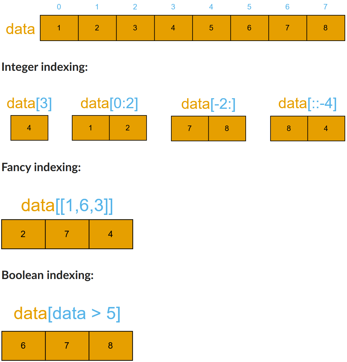
Array indexing
Basic indexing is similar to Python lists. Note that advanced indexing creates copies of arrays.
# 1D example

import numpy as np

data = np.array([1,2,3,4,5,6,7,8])

# integer indexing
print("Integer indexing")
print(f"data = {data}")
print(f"data[3] = {data[3]}")
print(f"data[0:2] = {data[0:2]}")
print(f"data[-2] = {data[-2]}")
print(f"data[::-4] = {data[::-4]}")

# fancy indexing
print("\nFancy indexing")
print(f"data[[1,6,3]] = {data[[1,6,3]]}")

# boolean indexing
print("\nBoolean indexing")
print(f"data[data>5] = {data[data>5]}")
Integer indexing
data = [1 2 3 4 5 6 7 8]
data[3] = 4
data[0:2] = [1 2]
data[-2] = 7
data[::-4] = [8 4]

Fancy indexing
data[[1,6,3]] = [2 7 4]

Boolean indexing
data[data>5] = [6 7 8]
Exercise
Run the code below to get familiar with indexing in a 2D example.
# 2D example

data = np.array([[1, 2, 3, 4],[5, 6, 7, 8],[9, 10, 11, 12]])

# integer indexing
print("Integer indexing")
print(f"data[1] = {data[1]}")
print(f"data[:, 1] = {data[:, 1]}")
print(f"data[1:3, 2:4] = {data[1:3, 2:4]}")

# fancy indexing
print("\nFancy indexing")
print(f"data[[0,2,1], [2,3,0]] = {data[[0,2,1], [2,3,0]]}")

# boolean indexing
print("\nBoolean indexing")
print(f"data[data>10] = {data[data>10]}")
Caution
Again, you should move the code above to a separate code block, or change its cell type from from Markdown to Code.
Array aggregation
Apart from aggregating values, one can also aggregate across rows or columns by using the axis parameter:
import numpy as np
data = np.array([[0, 1, 2], [3, 4, 5]])
data.max()
np.int64(5)
data.sum()
np.int64(15)
data.min(axis=0)
array([0, 1, 2])
data.min(axis=1)
array([0, 3])
Array reshaping
Sometimes, you need to change the dimension of an array. One of the most common need is to transposing the matrix during the dot product. Switching the dimensions of a NumPy array is also quite common in more advanced cases.
import numpy as np
data = np.array([1,2,3,4,5,6,7,8,9,10,11,12])
data.reshape(4,3)
array([[ 1,  2,  3],
       [ 4,  5,  6],
       [ 7,  8,  9],
       [10, 11, 12]])
data.reshape(3,4)
array([[ 1,  2,  3,  4],
       [ 5,  6,  7,  8],
       [ 9, 10, 11, 12]])
Views and copies of arrays
Simple assignment creates references to arrays
Slicing creates views to the arrays
Use
copyfor real copying of arrays
a = np.arange(10)
b = a              # reference, changing values in b changes a
b = a.copy()       # true copy

c = a[1:4]         # view, changing c changes elements [1:4] of a
c = a[1:4].copy()  # true copy of subarray
I/O with NumPy
Numpy provides functions for reading from/writing to files. Both ASCII and binary formats are supported with the CSV and npy/npz formats.
CSV
The numpy.loadtxt() and numpy.savetxt() functions can be used. They save in a regular column layout and can deal with different delimiters, column titles and numerical representations.
a = np.array([1, 2, 3, 4])
np.savetxt("my_array.csv", a)
b = np.loadtxt("my_array.csv")

print(a == b)
[ True True True True]
Attention
If you get an eror like xxx, you should import numpy before the first line import numpy as np.
Binary
The npy format is a binary format used to dump arrays of any shape. Several arrays can be saved into a single npz file, which is simply a zipped collection of different npy files. All the arrays to be saved into a npz file can be passed as kwargs to the numpy.savez() function. The data can then be recovered using the numpy.load() method, which returns a dictionary-like object in which each key points to one of the arrays.
a = np.array([1, 2, 3, 4])
b = np.array([5, 6, 7, 8])

np.savez("my_arrays.npz", array_1=a, array_2=b)
data = np.load("my_arrays.npz")

print(data['array_1'] == a) # [ True  True  True  True]
print(data['array_2'] == b) # [ True  True  True  True]
[ True  True  True  True]
[ True  True  True  True]
Random numbers
The module numpy.random provides several functions for constructing random arrays
random(): uniform random numbersnormal(): normal distributionchoice(): random sample from given array…
print(np.random.random((2,2)),'\n')
[[0.14400948 0.48133518]
 [0.63105809 0.86880755]]
print(np.random.choice(np.arange(4), 10))
[2 3 0 3 0 0 2 0 1 1]
Warning
You might get different results from the above code example.
Polynomials
Polynomial is defined by an array of coefficients p
p(x, N) = p[0] x^{N-1} + p[1] x^{N-2} + ... + p[N-1]For example:
Least square fitting: :meth:
numpy.polyfitEvaluating polynomials: :meth:
numpy.polyvalRoots of polynomial: :meth:
numpy.roots
x = np.linspace(-4, 4, 7)
y = x**2 + rnd.random(x.shape)

p = np.polyfit(x, y, 2)
p
# array([ 0.96869003, -0.01157275, 0.69352514])
---------------------------------------------------------------------------
NameError                                 Traceback (most recent call last)
Cell In[19], line 2
      1 x = np.linspace(-4, 4, 7)
----> 2 y = x**2 + rnd.random(x.shape)
      3
      4 p = np.polyfit(x, y, 2)
      5 p

NameError: name 'rnd' is not defined
Linear algebra
NumPy can calculate matrix and vector products efficiently: :meth:
dot, :meth:vdot, …Eigenproblems: :meth:
linalg.eig, :meth:linalg.eigvals, …Linear systems and matrix inversion: :meth:
linalg.solve, :meth:linalg.inv
A = np.array(((2, 1), (1, 3)))
B = np.array(((-2, 4.2), (4.2, 6)))
C = np.dot(A, B)

b = np.array((1, 2))
np.linalg.solve(C, b) # solve C x = b
# array([ 0.04453441, 0.06882591])
Normally, NumPy utilises high performance libraries in linear algebra operations
Example: matrix multiplication C = A * B matrix dimension 1000
pure python: 522.30 s
naive C: 1.50 s
numpy.dot: 0.04 s
library call from C: 0.04 s
Pandas
Pandas is a Python package that provides high-performance and easy to use data structures and data analysis tools. The core data structures of Pandas are Series and Dataframes.
a Pandas
seriesis a one-dimensional NumPy array with an index which we could use to access the dataa
dataframeconsist of a table of values with labels for each row and column. A dataframe can combine multiple data types, such as numbers and text, but the data in each column is of the same type.each column of a dataframe is a series object - a dataframe is thus a collection of series.

Data analysis workflow
Pandas is a powerful tool for many steps of a data analysis pipeline:
To explore some of the capabilities, we start with an example dataset containing the passenger list from the Titanic, which is often used in Kaggle competitions and data science tutorials. First step is to load Pandas and download the dataset into a dataframe.
import pandas as pd

url = "https://raw.githubusercontent.com/pandas-dev/pandas/master/doc/data/titanic.csv"

# set the index to the "Name" column
titanic = pd.read_csv(url, index_col="Name")
Note
Pandas also understands multiple other formats, for example read_excel(), read_hdf(), read_json(), etc. (and corresponding methods to write to file: to_csv(), to_excel(), to_hdf(), to_json(), …)…)
We can now view the dataframe to get an idea of what it contains and print some summary statistics of its numerical data:
# print the first 5 lines of the dataframe
print(titanic.head())

# print some information about the columns
print(titanic.info())

# print summary statistics for each column
print(titanic.describe())
Missing/invalid data
What if your dataset has missing data? Pandas uses the value np.nan to represent missing data, and by default does not include it in any computations. We can find missing values, drop them from our dataframe, replace them with any value we like or do forward or backward filling.
titanic.isna()                           # returns boolean mask of NaN values

print(titanic.dropna())                  # drop missing values
print(titanic.dropna(how="any"))         # or how="all"
print(titanic.dropna(subset=["Cabin"]))  # only drop NaNs from one column
print(titanic.fillna(0))                 # replace NaNs with zero
Data wrangling operations
Begin by defining a new dataframe:
import numpy as np
import pandas as pd
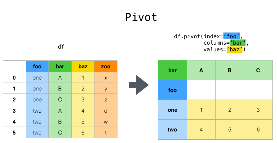
df = pd.DataFrame(
{
"foo": ["one", "one", "one", "two", "two", "two"] ,
"bar": ["A", "B", "C"] * 2,
"baz": np.linspace(1,6,6).astype(int),
"zoo": ["x","y","z","q","w","t"]
}
)
df
Suppose we would like to represent the table in such a way that
the columns are the unique variables from “bar” and the index from “foo”.
To reshape the data into this form, we use the :meth:DataFrame.pivot
method (also implemented as a top level function :func:~pandas.pivot):
pivoted = df.pivot(index="foo", columns="bar", values="baz")
pivoted
Note
entries, cannot reshape`` if the index/column pair is not unique. In this
case, consider using :func:~pandas.pivot_table which is a generalization
of pivot that can handle duplicate values for one index/column pair.
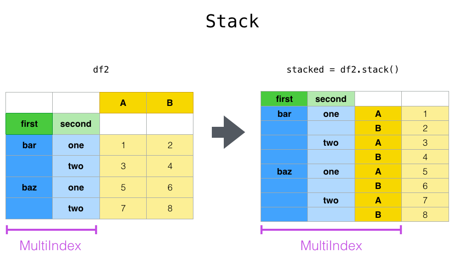
Stacking and unstacking
Closely related to the :meth:pivot method are the related
:meth:stack and :meth:unstack methods available on Series and DataFrame.
These methods are designed to work together with MultiIndex objects.
The :meth:stack function “compresses” a level in the DataFrame columns to produce either:
A Series, in the case of a simple column Index.
A DataFrame, in the case of a MultiIndex in the columns.
If the columns have a MultiIndex, you can choose which level to stack. The stacked level becomes the new lowest level in a MultiIndex on the columns:
tuples = list(zip(*[
        ["bar", "bar", "baz", "baz", "foo", "foo", "qux", "qux"],
        ["one", "two", "one", "two", "one", "two", "one", "two"],
              	   ]))
columns = pd.MultiIndex.from_tuples([
        ("bar", "one"),
        ("bar", "two"),
        ("baz", "one"),
        ("baz", "two"),
        ("foo", "one"),
        ("foo", "two"),
        ("qux", "one"),
        ("qux", "two"),
   ],
   names=["first", "second"])
index = pd.MultiIndex.from_tuples(tuples, names=["first", "second"])
Note
there are other ways to generate MultiIndex, e.g.
index = pd.MultiIndex.from_product(
    [("bar", "baz", "foo", "qux"), ("one", "two")], names=["first", "second"]
)

df = pd.DataFrame(np.linspace(1,16,16).astype(int).reshape(8,2), index=index, columns=["A", "B"])
df
df2 = df[:4]
df2
stacked=df2.stack()
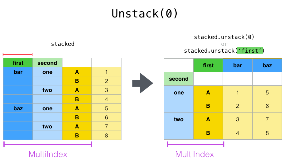
The unstack() method performs the inverse operation of stack(), and by default unstacks the last level. If the indexes have names, you can use the level names instead of specifying the level numbers.
stacked.unstack()
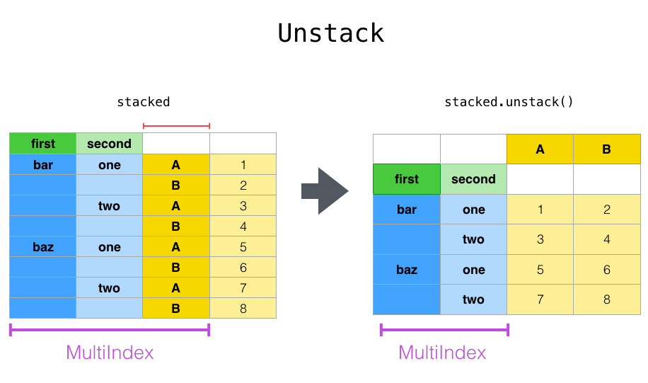
stacked.unstack(1)
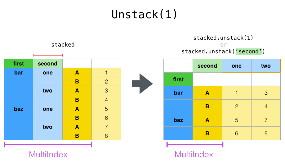
or
stacked.unstack("second")
Aggregation
Here we will go through the following example
import urllib.request
import pandas as pd

header_url = 'ftp://ftp.ncdc.noaa.gov/pub/data/uscrn/products/daily01/HEADERS.txt'
with urllib.request.urlopen(header_url) as response:
    data = response.read().decode('utf-8')
lines = data.split('\n')
headers = lines[1].split(' ')

ftp_base = 'ftp://ftp.ncdc.noaa.gov/pub/data/uscrn/products/daily01/'
dframes = []
for year in range(2016, 2019):
    data_url = f'{year}/CRND0103-{year}-NY_Millbrook_3_W.txt'
    df = pd.read_csv(ftp_base + data_url, parse_dates=[1],
                     names=headers,header=None, sep='\s+',
      	             na_values=[-9999.0, -99.0])
    dframes.append(df)

df = pd.concat(dframes)
df = df.set_index('LST_DATE')
df.head()
df['T_DAILY_MEAN'] # or df.T_DAILY_MEAN
df['T_DAILY_MEAN'].aggregate([np.max,np.min,np.mean])
df.index   # df.index is a pandas DateTimeIndex object.
gbyear=df.groupby(df.index.year)
gbyear.T_DAILY_MEAN.head()
gbyear.T_DAILY_MEAN.max()
gbyear.T_DAILY_MEAN.aggregate(np.max)
gbyear.T_DAILY_MEAN.aggregate([np.min, np.max, np.mean, np.std])
now let us calculate the monthly mean values
gb=df.groupby(df.index.month)
df.groupby('T_DAILY_MEAN')  # or  df.groupby(df.T_DAILY_MEAN)
monthly_climatology = df.groupby(df.index.month).mean()
monthly_climatology
Each row in this new dataframe respresents the average values for the months (1=January, 2=February, etc.)
monthly_T_climatology = df.groupby(df.index.month).aggregate({'T_DAILY_MEAN': 'mean',
                                                            'T_DAILY_MAX': 'max',
                                                            'T_DAILY_MIN': 'min'})
monthly_T_climatology.head()
daily_T_climatology = df.groupby(df.index.dayofyear).aggregate({'T_DAILY_MEAN': 'mean',
                                                            'T_DAILY_MAX': 'max',
                                                            'T_DAILY_MIN': 'min'})
def standardize(x):
    return (x - x.mean())/x.std()
anomaly = df.groupby(df.index.month).transform(standardize)
Transformation
The key difference between aggregation and transformation is that aggregation returns a smaller object than the original, indexed by the group keys, while transformation returns an object with the same index (and same size) as the original object.
In this example, we standardize the temperature so that the distribution has zero mean and unit variance. We do this by first defining a function called standardize and then passing it to the transform method.
transformed = df.groupby(lambda x: x.year).transform(
    lambda x: (x - x.mean()) / x.std()
)
grouped = df.groupby(lambda x: x.year)
grouped_trans = transformed.groupby(lambda x: x.year)
Scipy
SciPy is a library that builds on top of NumPy. It contains a lot of interfaces to battle-tested numerical routines written in Fortran or C, as well as Python implementations of many common algorithms.
Let us look more closely into one out of the countless useful functions available in SciPy. curve_fit() is a non-linear least squares fitting function. NumPy has least-squares fitting via the np.linalg.lstsq() function, but we need to go to SciPy to find non-linear curve fitting. This example fits a power-law to a vector.
import numpy as np
from scipy.optimize import curve_fit

def powerlaw(x, A, s):
    return A * np.power(x, s)

# data
Y = np.array([9115, 8368, 7711, 5480, 3492, 3376, 2884, 2792, 2703, 2701])
X = np.arange(Y.shape[0]) + 1.0

# initial guess for variables
p0 = [100, -1]
# fit data
params, cov = curve_fit(f=powerlaw, xdata=X, ydata=Y, p0=p0, bounds=(-np.inf, np.inf))

print("A =", params[0], "+/-", cov[0,0]**0.5)
print("s =", params[1], "+/-", cov[1,1]**0.5)
# optionally plot
import pandas as pd
import hvplot.pandas

data = pd.DataFrame({
    "x": X,
    "raw data": Y,
    "power law": powerlaw(X, params[0], params[1])
})
scatter = data["raw data"].hvplot(kind="scatter", color="red")
line = data["power law"].hvplot()
(scatter * line)
Exercises
Working effectively with dataframes
Recall the curve_fit() method from SciPy discussed above, and imagine that we want to fit powerlaws to every row in a large dataframe. How can this be done effectively?
First define the powerlaw() function and another function for fitting a row of numbers:
import numpy as np
import pandas as pd
from scipy.optimize import curve_fit

def powerlaw(x, A, s):
    return A * np.power(x, s)

def fit_powerlaw(row):
    X = np.arange(row.shape[0]) + 1.0
    params, cov = curve_fit(f=powerlaw, xdata=X, ydata=row, p0=[100, -1], bounds=(-np.inf, np.inf))
    return params[1]
Next load a dataset with multiple rows similar to the one used in the example above:
df = pd.read_csv("https://raw.githubusercontent.com/ENCCS/hpda-python/main/content/data/results.csv")
# print first few rows
df.head()
Now consider these four different ways of fitting a powerlaw to each row of the dataframe:
# 1. Loop

powers = []
for row_indx in range(df.shape[0]):
    row = df.iloc[row_indx,1:]
    p = fit_powerlaw(row)
    powers.append(p)
# 2. `iterrows()

powers = []
for row_indx,row in df.iterrows():
    p = fit_powerlaw(row[1:])
    powers.append(p)
# 3. `apply()

powers = df.iloc[:,1:].apply(fit_powerlaw, axis=1)
# 4. `apply()` with `raw=True`

# raw=True passes numpy ndarrays instead of series to fit_powerlaw
powers = df.iloc[:,1:].apply(fit_powerlaw, axis=1, raw=True)
Which one do you think is most efficient? You can measure the execution time by adding %%timeit to the first line of a Jupyter code cell. More on timing and profiling in a later episode.
Solution
The execution time for four different methods are described below. Note that you may get different numbers when you run these examples.
# 1 Loop

%%timeit
powers = []
for row_indx in range(df.shape[0]):
   row = df.iloc[row_indx,1:]
   p = fit_powerlaw(row)
   powers.append(p)

# 33.6 ms ± 682 µs per loop (mean ± std. dev. of 7 runs, 10 loops each)
# 2. `iterrows()`

%%timeit
powers = []
for row_indx,row in df.iterrows():
   p = fit_powerlaw(row[1:])
   powers.append(p)

# 28.7 ms ± 947 µs per loop (mean ± std. dev. of 7 runs, 10 loops each)
# 3. `apply()`

%%timeit
powers = df.iloc[:,1:].apply(fit_powerlaw, axis=1)

# 26.1 ms ± 1.19 ms per loop (mean ± std. dev. of 7 runs, 10 loops each)
# 4. `apply()` with `raw=True`

%%timeit
powers = df.iloc[:,1:].apply(fit_powerlaw, axis=1, raw=True)

# 24 ms ± 1.27 ms per loop (mean ± std. dev. of 7 runs, 10 loops each)
Further analysis of Titanic passenger list dataset
Consider the titanic dataset.
If you haven’t done so already, load it into a dataframe before the exercises:
import pandas as pd; url = "https://raw.githubusercontent.com/pandas-dev/pandas/master/doc/data/titanic.csv"; titanic = pd.read_csv(url, index_col="Name")
Compute the mean age of the first 10 passengers by slicing and the
meanmethodUsing boolean indexing, compute the survival rate (mean of “Survived” values) among passengers over and under the average age. Now investigate the family size of the passengers (i.e. the “SibSp” column):
What different family sizes exist in the passenger list?
Hint: try the
unique()method
What are the names of the people in the largest family group?
(Advanced) Create histograms showing the distribution of family sizes for passengers split by the fare, i.e. one group of high-fare passengers (where the fare is above average) and one for low-fare passengers
Hint: instead of an existing column name, you can give a lambda function as a parameter to
histto compute a value on the fly. For examplelambda x: "Poor" if titanic["Fare"].loc[x] < titanic["Fare"].mean() else "Rich").
Solution
Mean age of the first 10 passengers:
titanic.iloc[:10,:]["Age"].mean()ortitanic.iloc[:10,4].mean()ortitanic.loc[:"Nasser, Mrs. Nicholas (Adele Achem)", "Age"].mean()
Survival rate among passengers over and under average age:
titanic[titanic["Age"] > titanic["Age"].mean()]["Survived"].mean()andtitanic[titanic["Age"] < titanic["Age"].mean()]["Survived"].mean()
Existing family sizes:
titanic["SibSp"].unique()Names of members of largest family(ies):
titanic[titanic["SibSp"] == 8].indextitanic.hist("SibSp", lambda x: "Poor" if titanic["Fare"].loc[x] < titanic["Fare"].mean() else "Rich", rwidth=0.9)
Keypoints
NumPy provides a static array data structure, fast mathematical operations for arrays and tools for linear algebra and random numbers
Pandas dataframes are a good data structure for tabular data
Dataframes allow both simple and advanced analysis in very compact form
SciPy contains a lot of interfaces to battle-tested numerical routines
Summary
In this lesson, we explored how efficient array computing enables high-performance numerical programming in Python. NumPy provides fast and memory-efficient array operations through vectorization, while Pandas builds on top of NumPy to offer powerful tools for structured data analysis. SciPy further extends these capabilities with advanced numerical algorithms.
By leveraging these libraries and avoiding inefficient Python loops, developers can write code that is both expressive and performant, making Python a strong choice for scientific computing and data-intensive applications.